Week 7
Survey Research

SOCI 316

Sakeef M. Karim
Amherst College

SOCIAL RESEARCH

What Surveys Can Do—
March 13^th

Help Us Draw Inferences

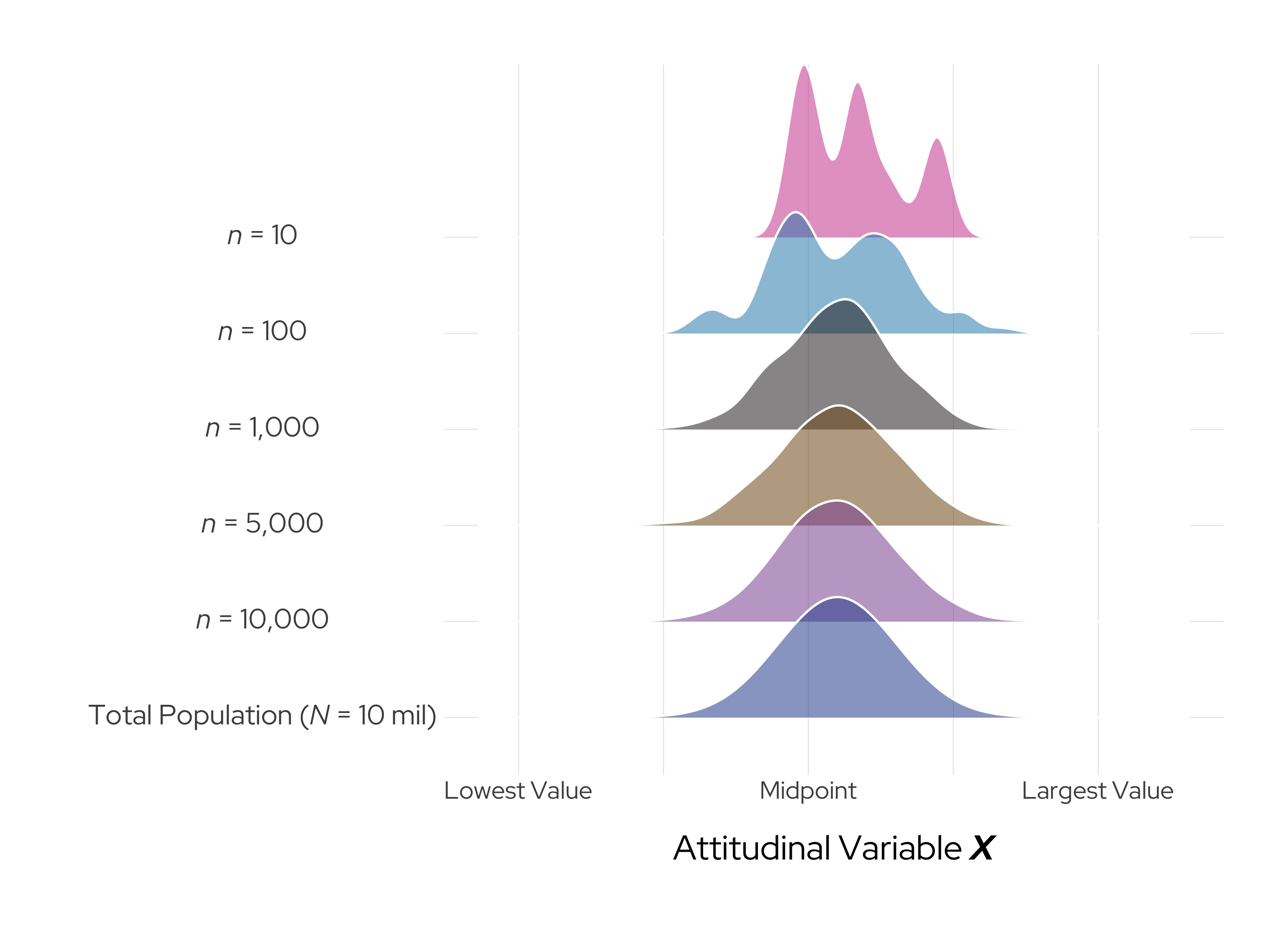
In the social sciences, we often want to know the characteristics of a population of interest. Yet collecting data from every individual in the target population may be prohibitively expensive or simply not feasible … In survey research, we collect data from a subset of observations in order to understand the target population as a whole.

(Llaudet and Imai 2023, 52, EMPHASIS ADDED)

Help Us Draw Inferences

A Reminder

Help Us Draw Inferences

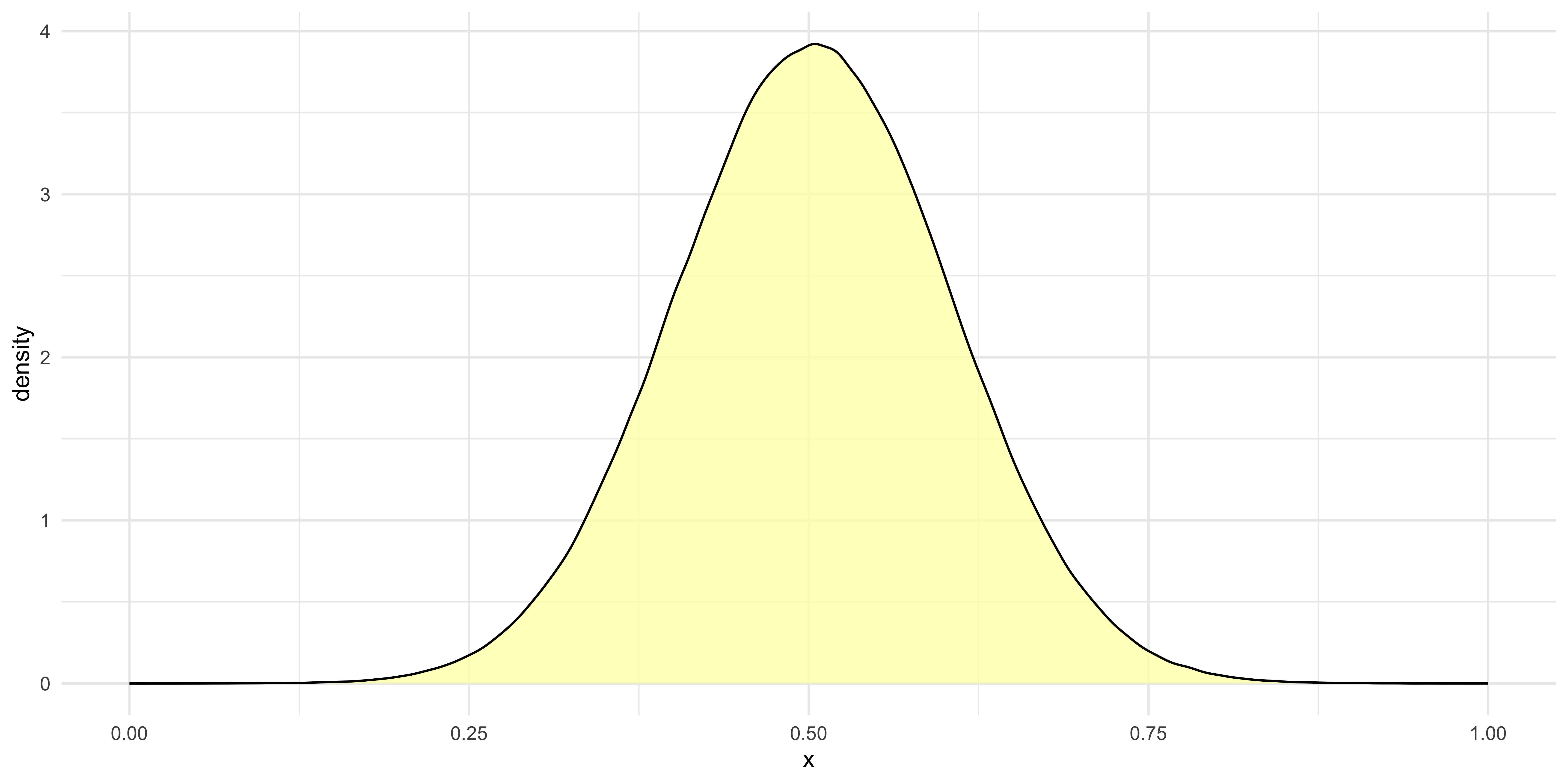
Total Population, N

library(tidyverse)

# Generating a population with one million people

set.seed(101)

population <- tibble(x = rnorm(1e6, mean = 0, sd = 27),
                     sample = "Overall") |> 
              mutate(x = scales::rescale(x, to = c(0, 1)))

ggplot(population, 
       mapping = aes(x = x)) +
geom_density(alpha = 0.75, fill = "#FFFFB3") +
theme_minimal() 

Help Us Draw Inferences

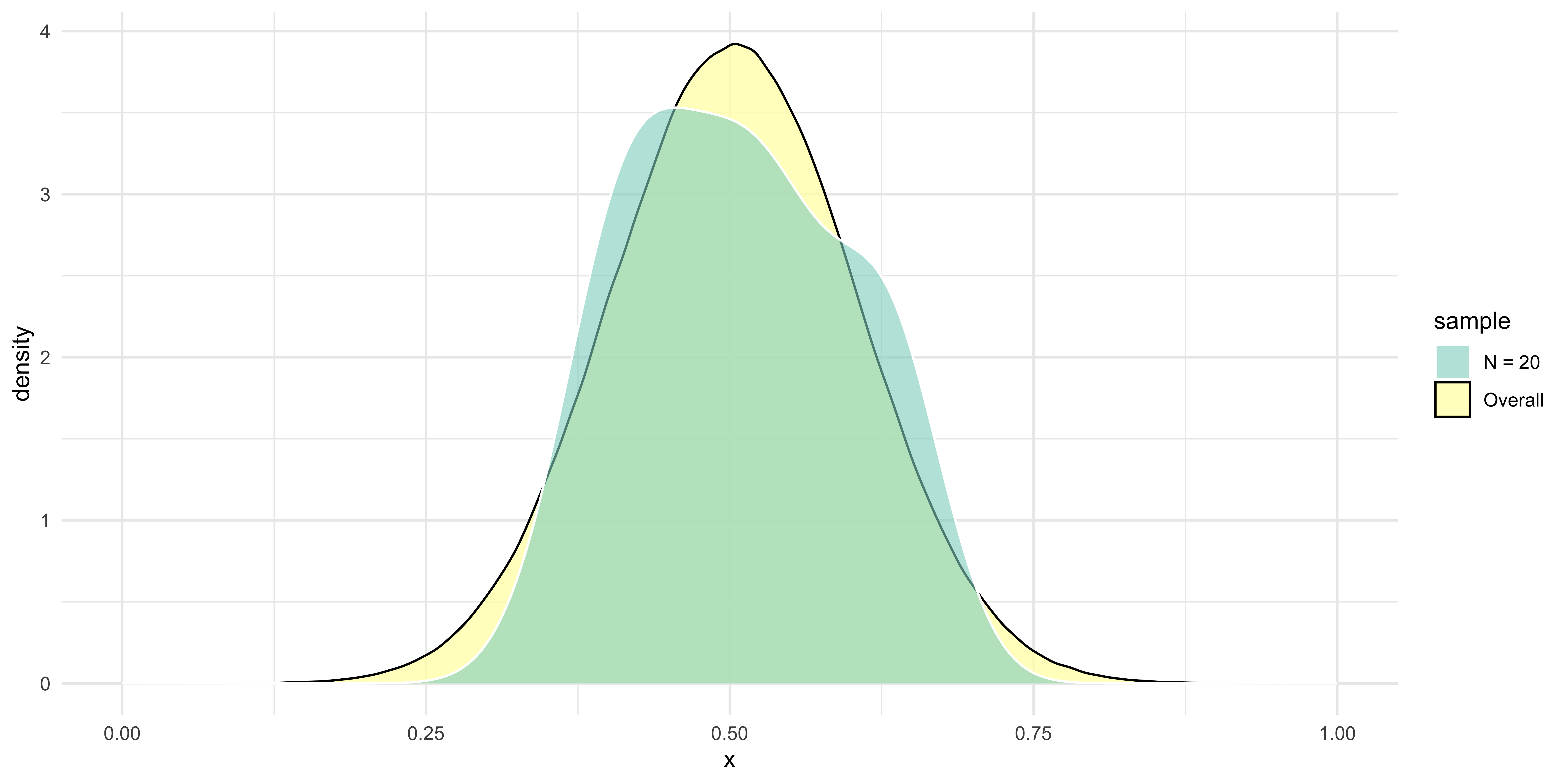
n = 20

set.seed(101)

ggplot(population, 
       mapping = aes(x = x, fill = sample)) +
geom_density(alpha = 0.75) +
geom_density(colour = "white",
             alpha = 0.6,
             data = population |> 
                    # Toggle these numbers on your own time! Try n = 10, 100, 1000, 5000
                    slice_sample(n = 20) |> 
                    mutate(sample = "N = 20")) +
theme_minimal() +
scale_fill_brewer(palette = "Set3")

Help Us Draw Inferences

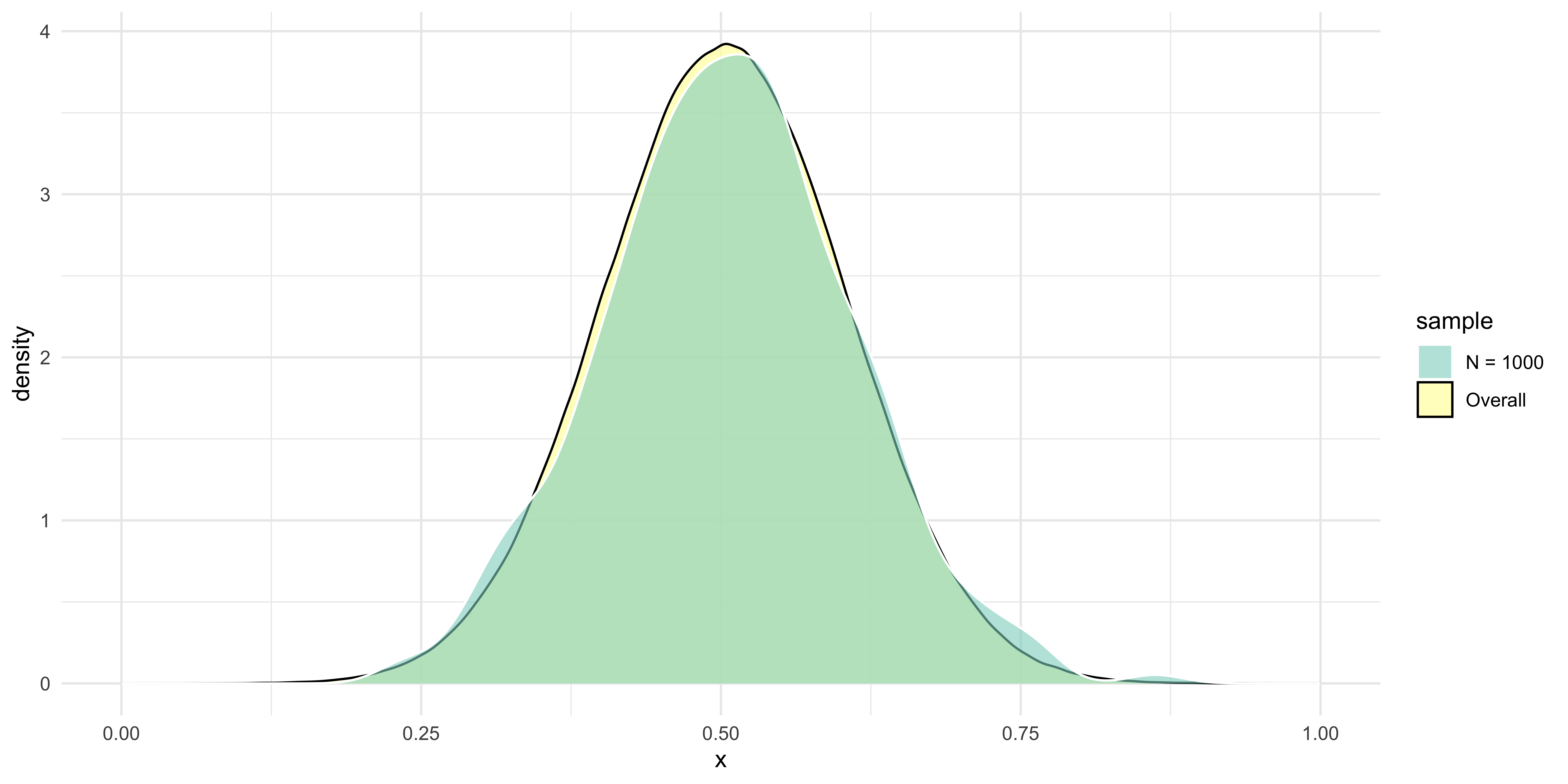
n = 1000

set.seed(101)

ggplot(population, 
       mapping = aes(x = x, fill = sample)) +
geom_density(alpha = 0.75) +
geom_density(colour = "white",
             alpha = 0.6,
             data = population |> 
                    # Toggle these numbers on your own time! Try n = 10, 100, 1000, 5000
                    slice_sample(n = 1000) |> 
                    mutate(sample = "N = 1000")) +
theme_minimal() +
scale_fill_brewer(palette = "Set3")

Help Us Draw Inferences

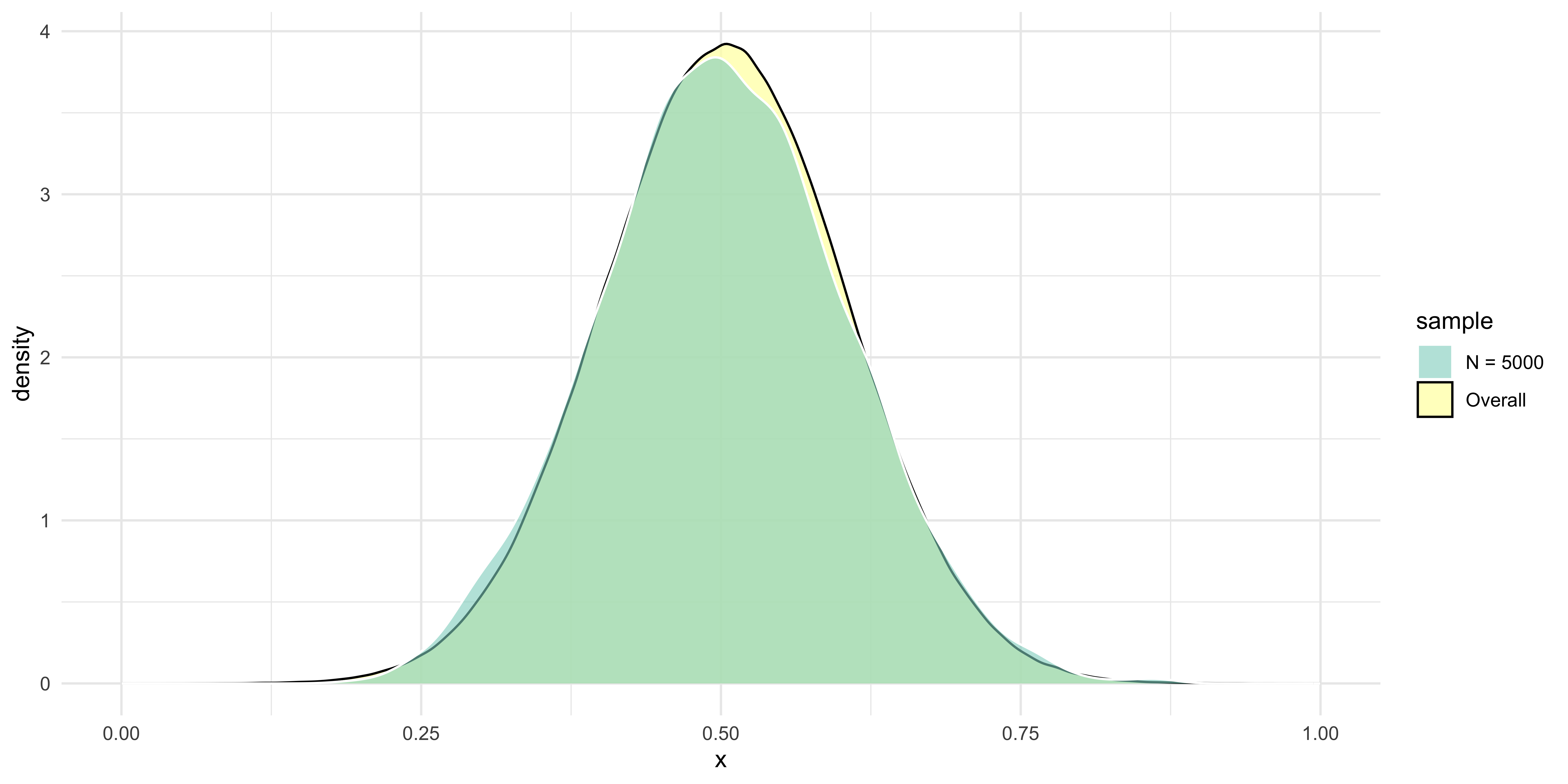
n = 5000

set.seed(101)

ggplot(population, 
       mapping = aes(x = x, fill = sample)) +
geom_density(alpha = 0.75) +
geom_density(colour = "white",
             alpha = 0.6,
             data = population |> 
                    # Toggle these numbers on your own time! Try n = 10, 100, 1000, 5000
                    slice_sample(n = 5000) |> 
                    mutate(sample = "N = 5000")) +
theme_minimal() +
scale_fill_brewer(palette = "Set3")

Sampling

Probability Samples

[W]hen we use random selection to determine the members of our sample, there is no systematic difference between the sample and the population from which it is drawn. Any differences are strictly due to random chance alone … Samples that are based on random selection are called probability samples. More precisely, a probability sample is one in which (a) random chance is used to select participants for the sample, and (b) each individual has a probability of being selected that can be calculated.

(Carr et al. 2020, 158, EMPHASIS ADDED)

Probability Samples

Of course, random sampling alone is not a panacea. Other considerations include—but are not limited to—our sample size,
n, and target population, U.

Consider the following list of potential respondents:

 [1] "Doering, Mikaleh"    "Neumiller, Kenneth"  "Cole, Drake"        
 [4] "Leathers, Nicole"    "Bail, Ryan"          "Williamson, Kelsey" 
 [7] "Ellwein, Charlotte"  "Konopka, Mark"       "Kenworthy, Keric"   
[10] "Balleydier, Shannon" "Fitzgibbons, Janey"  "Greco, Alexis"      
[13] "Ziegler, Bradley"    "Engelken, Autumn"    "Alhilo, Charlotte"  
[16] "Stump, Andrea"       "Kleppe, Ryan"        "Glide, Matthew"     
[19] "Jimenez, Ryan"       "Musk, Elon"         

Let’s say we want to talk to two of our respondents. Through random sampling, we might end up with this duo—

set.seed(905)
c(randomNames::randomNames(19, ethnicity = 5), "Musk, Elon") |> 
sample(size = 2)

[1] "Jimenez, Ryan" "Musk, Elon"   

Probability Samples

A Question

What is a sampling frame?

Probability Samples

Three Key Techniques

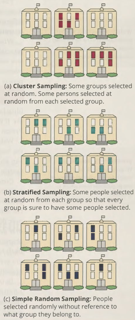
Figure 6.2 from Carr and colleagues (2020).

Probability Samples

Three Key Techniques

• Simple Random Sampling
• Cluster Sampling
• Stratified Sampling

A simple random sample has two key features. First, each individual has the same probability of being selected into the sample. Second—and this is the tricky part—each pair of individuals has the same probability of being selected.

(Carr et al. 2020, 164, EMPHASIS ADDED)

library(palmerpenguins)

penguins |> filter(year == max(year)) |> 
            slice_sample(n = 3)

# A tibble: 3 × 8
  species   island    bill_length_mm bill_depth_mm flipper_length_mm body_mass_g
  <fct>     <fct>              <dbl>         <dbl>             <int>       <int>
1 Adelie    Torgersen           39            17.1               191        3050
2 Gentoo    Biscoe              NA            NA                  NA          NA
3 Chinstrap Dream               45.7          17                 195        3650
# ℹ 2 more variables: sex <fct>, year <int>

In cluster sampling, the target population is first divided into groups, called clusters. Some of these clusters are selected at random. Then, some individuals are selected at random from within each cluster.

(Carr et al. 2020, 165, EMPHASIS ADDED)

set.seed(905)

two_islands <- penguins |> distinct(island) |>  
                           slice_sample(n = 2) |> 
                           pull(1)

penguins |> 
filter(island %in% two_islands) |> 
slice_sample(n = 2, by = island)

# A tibble: 4 × 8
  species island    bill_length_mm bill_depth_mm flipper_length_mm body_mass_g
  <fct>   <fct>              <dbl>         <dbl>             <int>       <int>
1 Adelie  Torgersen           40.9          16.8               191        3700
2 Adelie  Torgersen           44.1          18                 210        4000
3 Adelie  Biscoe              37.9          18.6               193        2925
4 Gentoo  Biscoe              47.2          13.7               214        4925
# ℹ 2 more variables: sex <fct>, year <int>

In stratified sampling, the population is divided into groups (called strata), and the researcher selects some members of every group.

(Carr et al. 2020, 166, EMPHASIS ADDED)

penguins |> 
slice_sample(prop = 0.03, by = island)

# A tibble: 9 × 8
  species   island    bill_length_mm bill_depth_mm flipper_length_mm body_mass_g
  <fct>     <fct>              <dbl>         <dbl>             <int>       <int>
1 Adelie    Torgersen           36.2          16.1               187        3550
2 Gentoo    Biscoe              49.1          14.5               212        4625
3 Gentoo    Biscoe              48.6          16                 230        5800
4 Gentoo    Biscoe              50.8          15.7               226        5200
5 Gentoo    Biscoe              45.1          14.4               210        4400
6 Adelie    Biscoe              40.5          18.9               180        3950
7 Chinstrap Dream               52            20.7               210        4800
8 Adelie    Dream               38.1          18.6               190        3700
9 Adelie    Dream               38.1          17.6               187        3425
# ℹ 2 more variables: sex <fct>, year <int>

A Note on Weighting

• The Intuition
• A Simple Example

In probability sampling, it is not a problem if some individuals have a higher likelihood of being in the sample than others, as long as we know what those probabilities are. If Person A is x times more likely to be in our sample than Person B, then we give Person A 1/x times as much weight as Person B when computing our estimates.

(Carr et al. 2020, 168, EMPHASIS ADDED)

Let’s say that s_share captures the distribution of islands in our sample, s, while u_share represents the distribution of islands in our target population, U.

# A tibble: 3 × 3
  island    s_share u_share
  <fct>       <dbl>   <dbl>
1 Biscoe      0.556   0.488
2 Dream       0.333   0.360
3 Torgersen   0.111   0.151

Now, here’s the weighted distribution of islands in s after applying weights:

set.seed(905)

dummy_sample <- penguins |> 
                slice_sample(prop = 0.03, by = island)

u_share <- penguins |> count(island) |> 
                       mutate(u_share = n/sum(n)) |> 
                       select(-n)

weights <- dummy_sample |> count(island) |> 
                           mutate(s_share = n/sum(n)) |> 
                           left_join(u_share) |> 
                           mutate(weight = u_share/s_share) |> 
                           select(island, weight)

dummy_sample |> left_join(weights) |> 
                count(island, wt = weight) |> 
                mutate(s_share = n/sum(n)) |> 
                select(-n)

# A tibble: 3 × 2
  island    s_share
  <fct>       <dbl>
1 Biscoe      0.488
2 Dream       0.360
3 Torgersen   0.151

Non-Representative Samples

Another Question

Are non-representative samples ever desirable?

Survey Research—
Formats, Delivery, etc.

Major Formats

Cross-Sectional v Panel Surveys

Adapted from Table 7.1 in Carr et al. (2020)

Characteristic	Cross-Sectional Surveys	Panel Surveys
Cost	Relatively low, as respondents are contacted only once	Relatively high, as respondents are contacted over time
Ease of Administration	Relatively easy	Relatively difficult
Causal Inference	Cannot ascertain causality clearly	Better suited to infer causality due to repeated measures
Sources of Bias	Typically exclude those difficult to reach	Same biases as cross-sectional surveys plus selective attrition
Ability to Document Change	Cannot assess within-person change	Well suited to assess within-person change over time
Attention to Social History	Cannot disentangle age, period, and cohort effects	Can partially disentangle age, period, and cohort effects if multiple cohorts included

Modes of Delivery

Strengths and Weaknesses

Adapted from Table 7.2 in Carr et al. (2020)

Attribute	Face-to-Face Interview	Mail or Self-Administered Questionnaire	Telephone Interview	Online Surveys
Cost	High	Low	Moderate	Low
Response Rate	High	Low	High	Moderate
Researcher Control Over Interview	High	Low	Moderate	Moderate
Interviewer Effects	High	Low	Moderate	Low

Error

Yet Another Question

What are some well-known sources of error (cf. Carr et al. 2020, 196) associated with survey research?

Class Exercise

Design Bad Survey Items

Get into groups of 2-3. Here are your tasks—

• Discuss–and review–the characteristics of high-quality survey questions (see Carr et al. 2020, 213–18).

• Design a set of five low quality (i.e., bad) questions.

• Exchange your questionnaire with another group.

• Try to identify the issues with the set of items you received.

Enjoy the Weekend

References

Carr, Deborah S., Elizabeth Heger Boyle, Benjamin Cornwell, Shelley J. Correll, Robert Crosnoe, Jeremy Freese, and Mary C. Waters. 2020. The Art and Science of Social Research. Second Edition. New York: W. W. Norton & Company, Inc.

Llaudet, Elena, and Kōsuke Imai. 2023. Data Analysis for Social Science: A Friendly and Practical Introduction. Princeton, NJ: Princeton University press.